Physics AI - The Illusion of Ground Truth

When you learn computational physics, one of the most challenging aspects is learning when to do, and when not to do something.

My doctoral research was largely in an area called “micromagnetics” which deals with how magnetic materials behave on small length scales (10s - 100s of nanometers). In micromagnetics, there is a governing partial differential equation called the Landau-Lifshitz-Gilbert equation, and a variety of energy terms that you can choose to include or exclude, depending on the material.

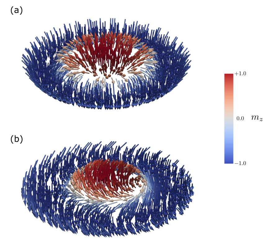
Some of these energy terms are always present in magnetic materials. Some of them are not. One in particular, which I dedicated a fair chunk of my life to thinking about is the demagnetising field, which describes how a magnetic material generates a field that opposes its own magnetism. When you go and simulate a magnetic material, there are a number of circumstances in which you can leave this term out. If the sample you are simulating is really thin, then you can replace the very expensive calculation with an approximate ‘anisotropic’ term. If the sample you’re simulating is really small, e.g. a nanoparticle small enough that it’s smaller than a characteristic length scale in which your particle doesn’t form a single magnetic region called a “domain”, then similarly we can neglect this term. But for the vast majority of systems, we do need to include it in simulations. Nonetheless, there have long been a series of relatively questionable papers in which it was neglected nonetheless.

This is not particularly specific to this niche area of magnetics research. Generally, there is a wide range of physical models for any problem, and an informed user must decide - in the regime I care about, what physics model is appropriate?

Stepping through time

Beyond this, we also have many other factors to consider. We often consider a distinction between “static” problems, in which we search for an equilibrium position - something at the lowest energy, etc. vs “dynamic” problems where the system is changing. Consider for example a bridge spanning a river. If the bridge is fixed in position and you place a load in the middle, you can work out the equilibrium and see what the bridge would look like with a relatively simple calculation. Dynamic problems are often more complicated - you need to model how people are walking across the bridge, cars are driving across and more. Again you can do a simulation of the displacement and stress of the bridge. Knowing when these simulations is important - look for example at the Millenium Bridge in London opened and then swiftly closed because of it’s oscillating.

Time integration of differential equations is tricky and there are many footguns. A prototypical example you are taught in any early undergraduate computational physics course is that of a planet orbiting a star. A naive approach is to write down the force equation:

$$ \mathbf{F} = m_{\text{planet}} \frac{d^2\mathbf{x}}{dt^2} = -\frac{G m_{\text{star}} m_{\text{planet}}}{|\mathbf{x}|^3} \mathbf{x} $$

This is a second order equation, so we split it into two first order equations, one for the position and one for the velocity:

$$ \frac{d\mathbf{x}}{dt} = \mathbf{v}, \qquad \frac{d\mathbf{v}}{dt} = \mathbf{a}(\mathbf{x}) = -\frac{G m_{\text{star}}}{|\mathbf{x}|^3} \mathbf{x} $$

The simplest way to step these forward in time is the “Euler” scheme. We replace each derivative with a finite difference over a small timestep $\Delta t$, and use the current position and velocity to calculate the next ones:

$$ \mathbf{x}_{n+1} = \mathbf{x}_{n} + \Delta t \, \mathbf{v}_{n} $$

$$ \mathbf{v}_{n+1} = \mathbf{v}_{n} + \Delta t \, \mathbf{a}(\mathbf{x}_{n}) $$

In code, this is just a few lines:

for n in range(n_steps):
    r = np.sqrt(x[0]**2 + x[1]**2)
    a = -GM * x / r**3
    x, v = x + dt * v, v + dt * a

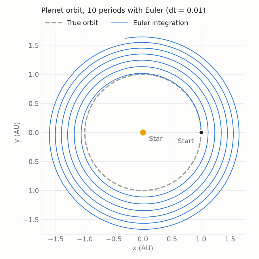
However this quickly fails as this plot shows:

If we plot the energy over time you can see that it isn’t conserved.

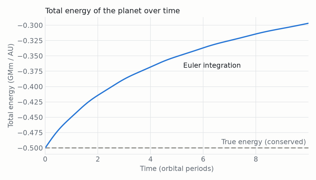
The planet gains a little bit of energy with every step, and it skirts out further and further away from the star. Making the timestep smaller slows this effect down at the expense of computational cost, but it never goes away - the error in each step always pushes the energy in the same direction, so it keeps on accumulating and drifting.

The fix here is not to throw more computing power at the problem, but to use a better integration scheme. A popular choice is “velocity Verlet” integration scheme:

$$ \mathbf{x}_{n+1} = \mathbf{x}_{n} + \Delta t \, \mathbf{v}_{n} + \frac{\Delta t^2}{2} \mathbf{a}(\mathbf{x}_{n}) $$

$$ \mathbf{v}_{n+1} = \mathbf{v}_{n} + \frac{\Delta t}{2} \left[ \mathbf{a}(\mathbf{x}_{n}) + \mathbf{a}(\mathbf{x}_{n+1}) \right] $$

Rather than updating the velocity using only the acceleration at the start of the step, it uses the average of the acceleration at the start and the end. In code it’s barely any longer than Euler, and because we can reuse the acceleration from the previous step, it still only needs one force calculation per step:

a = -GM * x / np.sqrt(x[0]**2 + x[1]**2)**3
for n in range(n_steps):
    x = x + dt * v + 0.5 * dt**2 * a
    r = np.sqrt(x[0]**2 + x[1]**2)
    a_new = -GM * x / r**3
    v = v + 0.5 * dt * (a + a_new)
    a = a_new

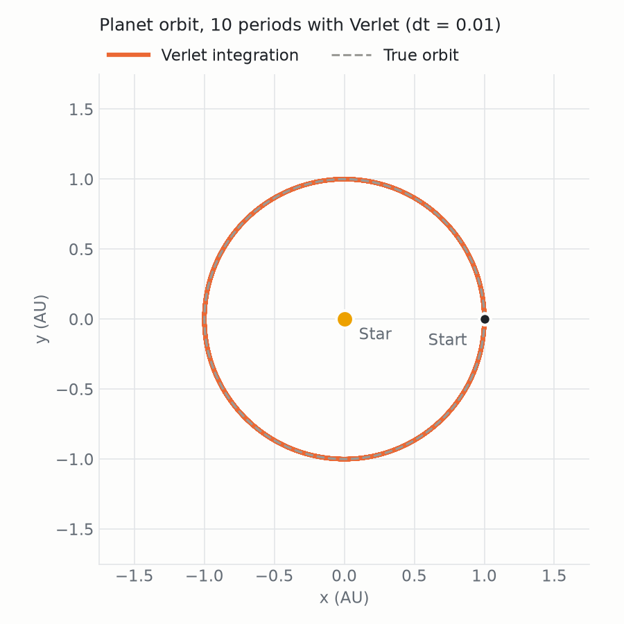
With exactly the same timestep, the planet now stays on its orbit:

and the energy no longer drifts:

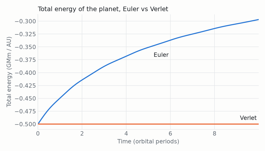
Verlet is an example of a “symplectic” integrator. Without going into too much detail, symplectic schemes enforce by construction the geometric structure of the equations of motion. In this case the relevant conserved quantity is energy, but other problems call for schemes that preserve other quantities - in micromagnetics for example, the conserved quantity is the magnitude of the magnetisation vector.

Which way does information flow?

Another factor is how information travels through a system when solving it. Take one of the simplest PDEs there is, the advection equation, which describes a quantity $u$ (say, the concentration of some dye in a pipe) being carried along at a constant speed $c$:

$$ \frac{\partial u}{\partial t} + c \frac{\partial u}{\partial x} = 0 $$

The exact solution is trivial. If the initial profile is $u(x, 0) = u_0(x)$, then for all later times:

$$ u(x, t) = u_0(x - ct) $$

Whatever shape you start with just slides along at speed $c$ without changing. Having an analytic solution like this is a luxury we rarely get, but it means we can see exactly how wrong a numerical scheme is. To solve it numerically, we put $u$ on a grid with spacing $\Delta x$ and need to approximate the spatial derivative. There are two obvious ways to do this with neighbouring points: use the point behind you, or the point in front of you:

$$ \text{Upwind:} \quad u_{i}^{n+1} = u_{i}^{n} - \frac{c \Delta t}{\Delta x} \left( u_{i}^{n} - u_{i-1}^{n} \right) $$

$$ \text{Downwind:} \quad u_{i}^{n+1} = u_{i}^{n} - \frac{c \Delta t}{\Delta x} \left( u_{i+1}^{n} - u_{i}^{n} \right) $$

On paper, these look equally reasonable - both are first order accurate approximations to the same derivative. In code, a single timestep of each differs only in which neighbour we use (the domain here is periodic, so the indices wrap around at the ends):

# Upwind: use the point behind
for i in range(n):
    u_new[i] = u[i] - c * dt / dx * (u[i] - u[i - 1])

# Downwind: use the point in front
for i in range(n):
    u_new[i] = u[i] - c * dt / dx * (u[(i + 1) % n] - u[i])

But the physics says that information flows in the direction of $c$. The upwind scheme takes its information from where the flow is coming from; the downwind scheme takes it from where the flow is going, which is information that physically can’t have arrived yet. Advecting a square pulse with both and comparing against the exact solution (dashed), the upwind scheme follows the pulse along, while the downwind scheme blows up - within twenty timesteps the solution has reached values of around 400:

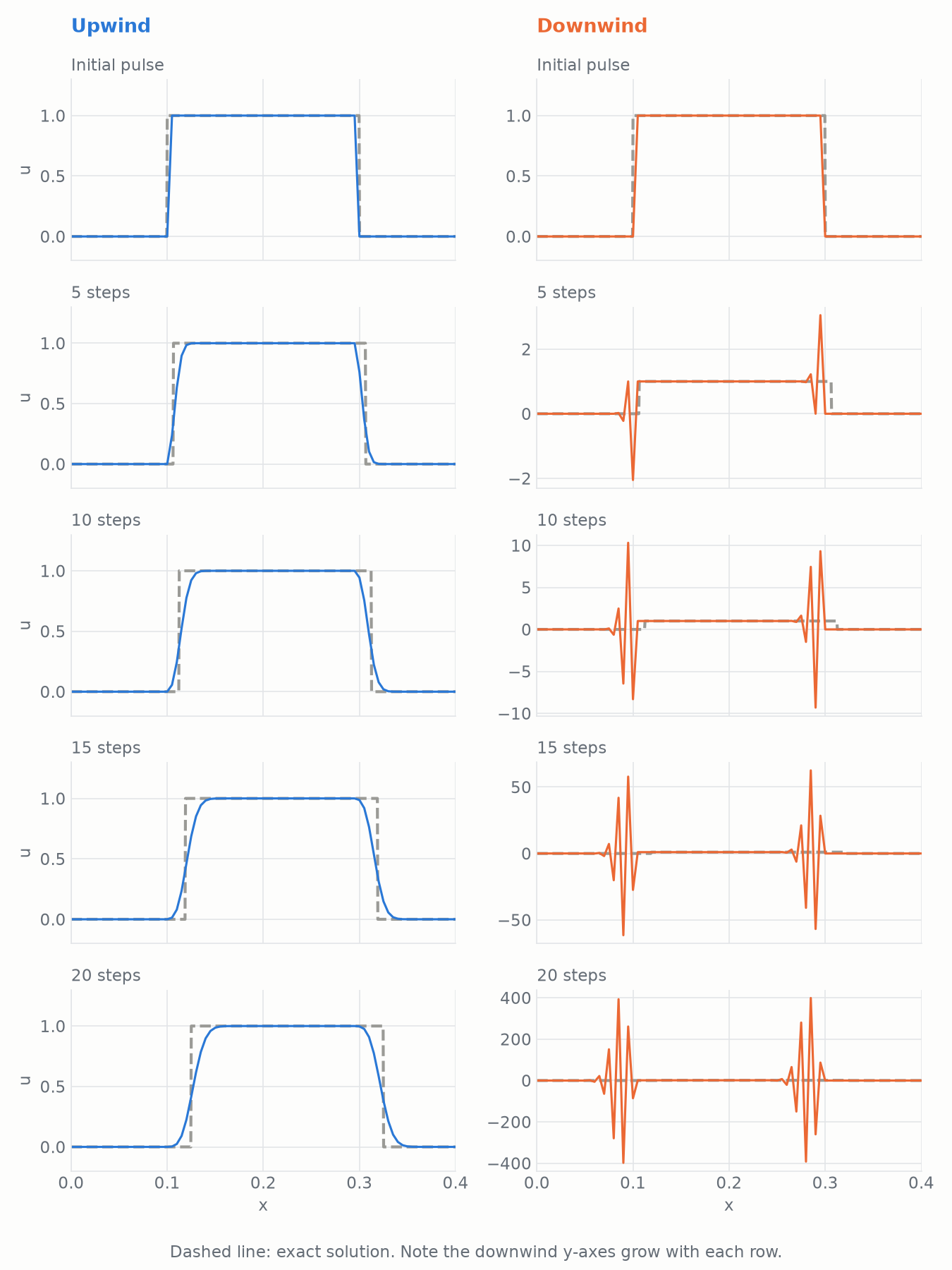
So upwind is the right answer? Not entirely. Look closely at the upwind column: the sharp edges of the pulse get a little softer with every row. Left to run for longer, the square pulse is smeared out into a smooth bump. The scheme is stable, but it has introduced “numerical diffusion” - the truncation error behaves like an extra diffusion term which isn’t in the equation we were trying to solve. Nothing has blown up, nothing looks obviously wrong, and if you didn’t know the answer in advance you may well believe this is what the physics does. This is the more dangerous kind of error. Fixing this needs a more sophisticated scheme, such as a “flux limited” scheme like van Leer’s, which keeps the edges sharp without blowing up.

Representing the geometry

Another choice one might make is in discretisation of physical space, and representing scalar and vector fields over that space. Typically you want to solve an equation on a “domain”. For example, one of the most prototypical partial differential equations is the Laplace equation:

$$ \nabla^2 \phi = \frac{\partial^2 \phi}{\partial x^2} + \frac{\partial^2 \phi}{\partial y^2} = 0 $$

which is used in modelling a large number of problems. Solving the Laplace equation on a square is easy - pretty much any technique can do this well. But solving it on a circular domain requires more thought.

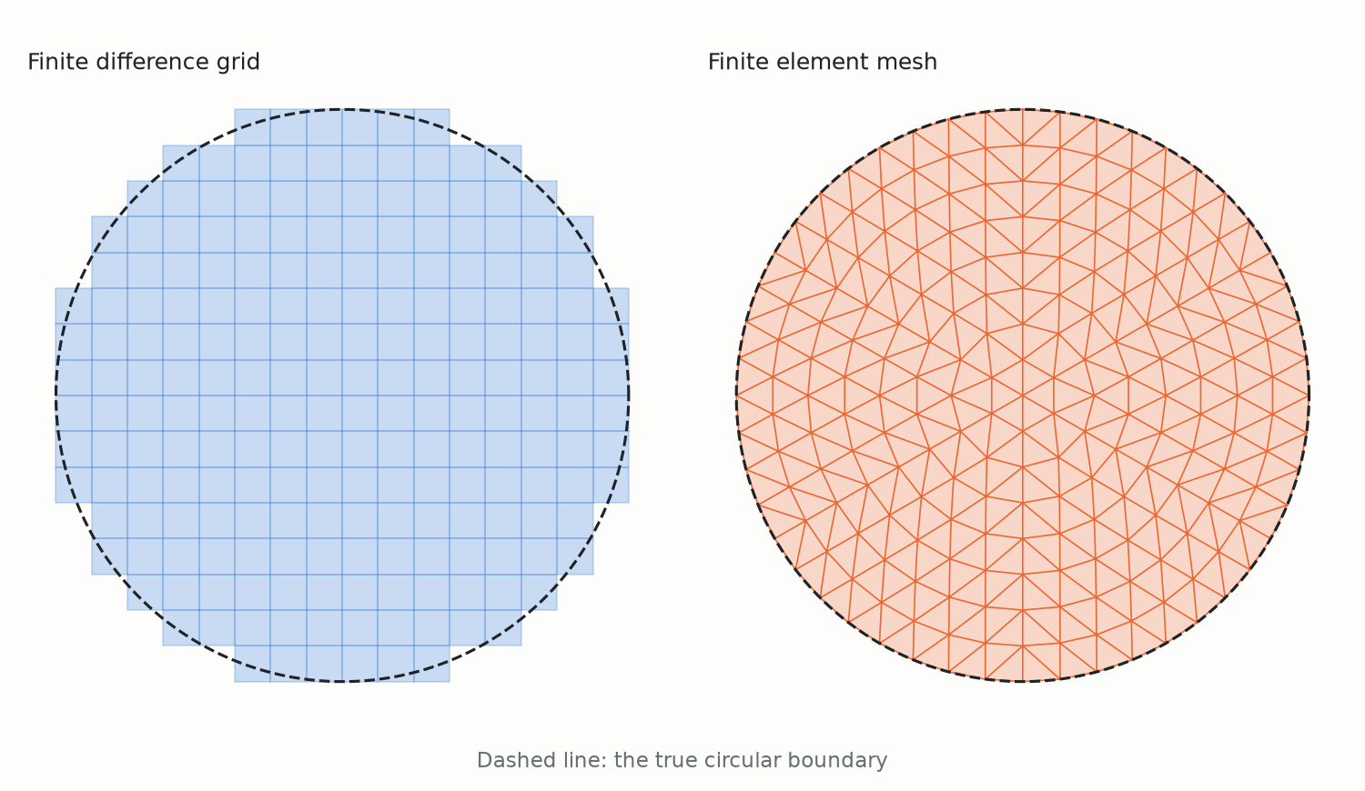
A finite difference scheme is easy to implement but leaves jagged edges representing the boundary unless the cell discretisation is really small. Finite elements, where the domain is broken up into a mesh of simple shapes (triangles or quadrilaterals in 2D, tetrahedra or hexahedra in 3D), allow a much more natural representation, because the elements can follow the boundary rather than approximating it with a staircase. This comes at the cost of a much more difficult to implement mathematical structure and a whole range of additional choices around basis functions, their order, support over the domain, and choices over continuity requirements - should the field be smooth i.e. no jumps allowed between elements? Should its derivative be smooth? Or even the tangential component between elements?

Even then, finite elements are far from the right tool for every problem. If the domain is infinite, as when calculating the field around a magnet or sound radiating from a loudspeaker, it’s often better to use the boundary element method, which only discretises the surface. In micromagnetics, the two are commonly combined. If the boundaries move, as with a heart valve or a flapping wing, remeshing every timestep becomes impractical, and immersed boundary methods lay the geometry over a fixed grid instead. Fluid dynamics is dominated by finite volume methods, which enforce the continuity equation exactly cell by cell, but problems with splashing free surfaces or materials that fragment are often tackled with very different particle based methods. Each of these brings its own set of choices, and its own ways to go wrong.

What this has to do with AI

So, the message here is that numerical methods are complicated. There are domain specific choices. They require knowledge of PDEs, the techniques used to solve them, and the choices inherent in them in what you are trying to model and why the method is appropriate. As much as knowing what to do, there is a lot of knowing what not to do.

Over the last year or so, I have really watched with interest the explosion of start up companies in particular who claim to have AI models trained on vast quantities of simulation data, which can make predictions about geometry changes and quickly return physical fields. I have watched this with some unease. In general, validation of simulations is not easy. It is actually easy to get wrong. Minor slip ups in choices of all of the above sorts of things can invalidate the results and make them non-physical. If you train a PINN or ’neural operator’, these models are great in the realm only where the original simulator was applicable, and even then, their architectures are known to have difficulty learning some components. This generalisability problem was also an issue with reduced order models, in which SVD decomposition of solutions dropped higher order modes in the solution, giving fast but confidently wrong answers.

My feeling is that it’s quite likely a lot of these companies are using “open codes” to generate data - OpenFOAM, CalculiX, etc. which are good tools but require much knowledge about the physics and maths, much more so than commercial solvers which generally try and guide people with “safety rails”. Alternatively, though, they might be the result of “vibe simming”. My own experiments with Claude Opus for e.g. though are that if you ask it a perfectly reasonable question:

“I want to model a steel beam under lots of loads. Write me a finite element code using FEniCSx for this problem.”

Then you end up almost always with the “lowest common denominator” simulator - e.g. in this case, the output was a simple linear stress/strain model with P1 tetrahedral elements, which give inaccurate displacements. This worries me a lot then, since simulation has never been “trusted” by everyone in every field and as I’ve tried to set out, nor should it. Often it can catastrophically fail to predict failure modes, especially where the physics evolves on very rapid timescales and steps out of the bounds of validity for that technique.

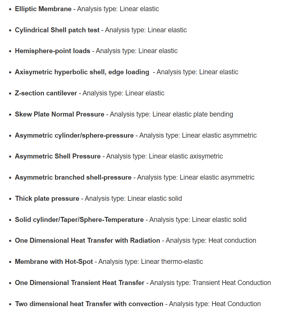
In various domains you have “standard problems” against which solvers are tested. For example, in finite element analysis, NAFEMS publish a series of benchmark results, which have surfaced over many years with blood, sweat and tears, normally when problems are found in various competing implementations of solid mechanics. In fluid dynamics people are commonly familiar with the lid-driven cavity. Even with this though, solvers handled by expert users with the problems set up correctly may pass these tests with flying colours, but it doesn’t mean that the same solver with the same settings applied to a different problem in the same domain is the right choice. It is interesting though that accompanying many claims of parametric design and simulation, we aren’t even seeing hints of testing against the full range of these standard problems.

The key thing that everyone in simulation and modelling has to remember is that we can have the most beautiful outputs in the world, but they can still be confidently wrong. We have to treat the validation case for AI models as the real world, not the simulation outputs. When we train a model on a simulator, it learns the simulator with all it’s choices and faults. This data is only an illusion of the ground truth.